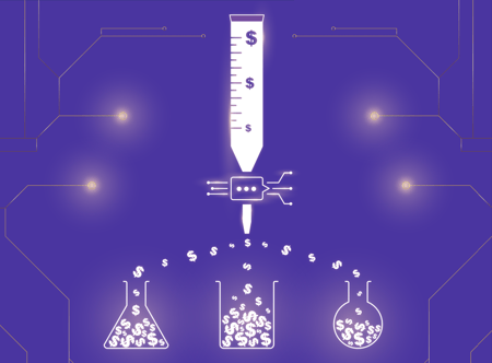
As promised in Lynx Analytics at Spark+AI Summit 2018, this is the first part of our series based on our SPARK+AI Summit presentation, How Neural Networks See Social Networks.
Let me introduce the ideas that the next posts will have in common: the graph convolutional network architecture and the benchmark datasets.
Graph Convolutional Networks
One problem that comes up often at Lynx is classifying vertices in a large graph. Practical examples would be guessing the gender of people in a social network, identifying compromised hosts in a computer network, or predicting who would be interested in an ad based on a phone call graph.
Different neural network architectures are suitable for dealing with different input formats. For our task we need one that can handle a graph as the input.
The very simplest neural network architecture is like this:
The input here is a feature vector: a fixed-length list of numbers. Graphs cannot be represented as a fixed-length list of numbers. Recurrent neural networks (RNNs) are used for taking variable-length input:
Each item of the variable-length input is a fixed-length feature vector. The network consumes the items one by one, updating an internal state after each item. (The state is also a fixed-length vector.)
This architecture is used for processing text (a sequence of characters or words) and voice (a sequence of sound samples). But a graph is not a sequence of things. It cannot be meaningfully ordered.
We can still use the same basic idea, with a twist:
Now we have a neural network in each vertex. We still do multiple iterations and update a state. But instead of the next item of a sequence, the network now gets the combined state vector of its neighbors each time. The input data (known vertex features and labels) is just put into the state vector at the start.
This architecture is called a graph convolutional network (GCN). I recommend Thomas Kipf’s 2016 article for anyone looking for more technical details and references. Lynx Analytics has used GCNs as the basis of much of our research. We find they can give highly accurate predictions on a variety of benchmark and real-world problems.
Our accuracy has improved gradually over the research. Early on it was annoying when hand-crafted solutions outperformed the neural network. Why would it not learn what we humans have managed to learn? But when the neural network overtook the hand-crafted solutions it was, surprisingly, even more annoying. What did it learn? Why wouldn’t it tell us? How could we understand the patterns in the data as well as the neural network does?
Explanations
Two commonly used approaches for understanding neural networks are feature visualization and attribution. As they both output some kind of explanation, it is a bit tricky to validate them. How do we know that the explanations are right?
The solution is to validate them on synthetic problems. We created two semi-synthetic datasets. In both cases the edges of the graph are a sample from a real-world social network dataset. But the vertex features are randomly picked. We call our single numeric feature “talent”, and vertices with a high talent are called “rockstars”. In the “three rockstar friends” task the vertices have a positive label if they have three or more rockstar friends:
Golden Pegs = Rockstars | Blue Vertices = Positive
Labels
In the “two steps from a rockstar” task the vertices have a positive label if they are exactly two steps away from a rockstar:
Golden Pegs = Rockstars | Blue Vertices = Positive
Labels
GCNs can be trained on these datasets to accurately reproduce the labels. Due to the synthetic nature of these datasets, we know exactly what rules the model has learned. If feature visualization and attribution can be used to recover these rules, they will also be able to recover the real-world rules in real-world datasets.
Coming up next: Feature Visualization on a GCN
Subscribe to our newsletter if you don’t want to miss the update!